lambda

Butterfly Effect and Hawkmoth Effect (II)

BX Pan

Recall of the Previous Post

In the previous post, I used the popular Lorenz System to illustrate the following ideas:

• Dynamic System
• Initial Sensitivity
• Temporal Mean
• Ensemble Mean

With these concepts constructed, I can explain the ideas of Butterfly Effect and Hawkmoth Effect, and their implications in “Climate Science”.

• Three body problem (Newtonian and General Relativity)

• Hierarchical modelling of Climate

This post tries to illustrate the idea of the limitation with numerical simulations(in Part I), followed by a discussion of its effects on the unstable foundation of “Climate Science“(in Part II).

The main features of dynamical systems theory (e.g. Smale, 1967; Arnol’d, 1983) that are important for the study of climate have been summarized by Ghil et al. (1991) and Ghil and Robertson (2000). T

The Climate System

The atmosphere has a characteristic time of days-to-weeks in terms of the life cycle of extratropical weather systems. The global mixing of atmospheric trace gases, on the other hand, takes one or more years. The meanders and rings of the major wind-driven currents are the oceanic counterpart of weather systems; their characteristic time is as short as months to years. Temperature and salinity contrasts, on the other hand, drive the oceans’ overturning circulation; its characteristic time is as long as centuries to millennia. Snow cover and sea ice have a huge seasonal cycle, as well as sub- and interannual variability, while continental ice sheets take many millennia to build up and at least centuries to collapse

Ensemble Forecast

The multiple simulations are conducted to account for the two usual sources of uncertainty in forecast models: (1) the errors introduced by the use of imperfect initial conditions, amplified by the chaotic nature of the evolution equations of the atmosphere, this is often referred to as sensitive dependence on the initial conditions; and (2) errors introduced because of imperfections in the model formulation, such as the approximate mathematical methods to solve the equations. Ideally, the verified future atmospheric state should fall within the predicted ensemble spread, and the amount of spread should be related to the uncertainty (error) of the forecast. In general, this approach can be used to make probabilistic forecasts of any dynamical system, and not just for weather prediction.

Toy Model – the Lorenz System

The Lorenz System is selected here for its rich exploration heritage. It is derived from the Oberbeck-Boussinesq Approximation to the equations describing fluid circulation in a shallow layer of fluid, heated uniformly from below and cooled uniformly from above. This fluid circulation is known as Rayleigh-Bénard Convection. The fluid is assumed to circulate in two dimensions (vertical and horizontal) with periodic rectangular boundary conditions(wikipedia). The system is described as follows:

Numerical Simulation

The equations can not be analytically integrated. A numerical simulator using Mathematica is coded as follows:

LorenzSystemSolution[x0_,y0_,z0_,a_;3,b_:26.5,c_:1]:=
Block[{x,y,z,t,tend,eq,init,xs,ys,zs},
	tend = 500;
	eq = { x'[t] == a (y[t] - x[t]), 
      	y'[t] == x[t] (b - z[t]) - y[t], 
      	z'[t] == x[t] y[t] - c z[t]};
	init = {x[0] == x0, y[0] == y0, z[0] == z0};
	{xs, ys, zs} = NDSolveValue[{eq , init}, {x, y, z}, {t, 0, tend},
		MaxSteps -> \[Infinity]];
	Table[{xs[t], ys[t], zs[t]}, {t, 0, tend}]]

I set the default parameters to a=3, b=26.5, c=1. There are many works considering the parameter settings and properties of the system. For those who are interested, Hirsch, Smale & Devaney, 2003 gives good supplements.

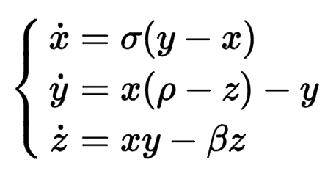
Given the initial condition, I can draw the trajectory of the dynamical system. For instance:

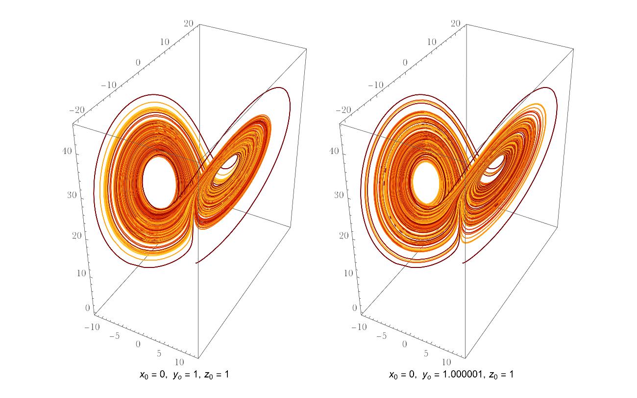
The initial x and z are identical for the two realizations, y differs slightly by 0.000001. It seems that the two trajectories are generally indistinguishable. But, if I compare the Euclidean Distance between the trajectories, for different magnitude of pertubations, the result is a little bit surprising:

Purtubations of different magnitude were added to initial y. For pertubations larger than 10^-16, we don’t need to wait too long before the divergence of the two trajectories. Similar things happen by tuning initial x or z. They diverge, then they never come back. The initial closeness does not guarantee likeliness forever. Just as marriage.

The divergent time here did not exceed 40 steps. It is reported that if we can initialize the Lorenz System with 4180 digit multiple precision, we can reach reliable simulation for 100000 steps, according to a 1200 CPU parallel simulation experiment(Shijun Liao, etc.. 2013).

Once the “realistic” and “simulated” trajectories start to diverge, the following realizations are evolving from distinct initials. This makes a determinisitic comparison meaningless. But does it mean that they provide no information?

What could Not be Achieved, Here Comes to Pass

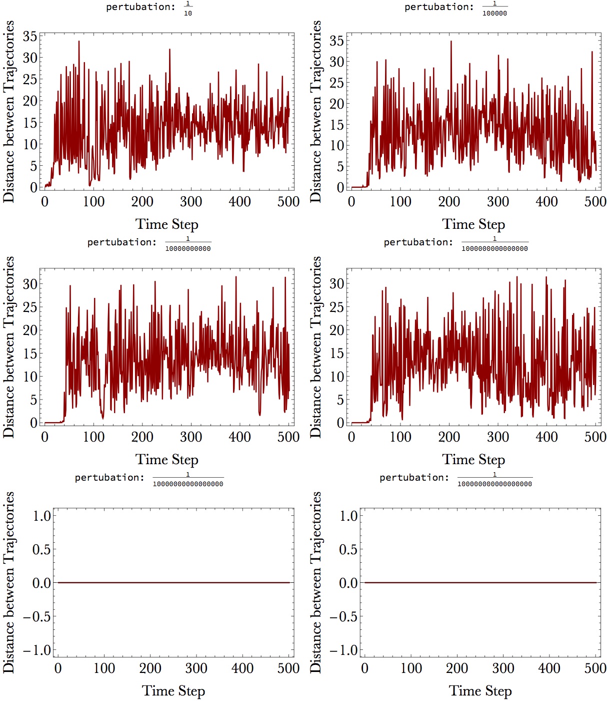
The general pattern of the trajectories above are quite alike although they are not close enough in the Euclidean Distance sense. A mathematical translation for the likeliness is that their temporal average location should be close. Below I do a uniform convolution over the trajectories to compare the temporal mean of them.

As the temporal resolution expands, the two trajectories are becoming more and more close in L2 sense. The local maximum divergence is due to the transition of phases(shown as two evolving centers). So, we can say that, in the long term mean sense, the system is predictable.

What no-one could Describe, Is Here Accomplished

It is natural to measure our understanding about a target variable/phenomenon with probability distribution. Even that we can not have a determinisitic estimation of initials, we do have a probabilistic estimation of it. While the determinisitc result can be proven to be false easily, the probabilistic one is always logically right since it’s a measuring of our mind rather than nature. We can feed the initial distribution to the dynamic system to reach the probability distribution of the trajectory. This is the idea behind ensemble forecast.

Assume that there is God in the Lorenz System. “He” is omniscient in observation, dynamical understanding and computing capacity(Roman, etc.. 2014). “He” knows that the system starts from (x=0,y=1,z=1) and follows the differential equation set perfectly. He can do simulation arbitrarily fast.

I, as the imperfect imitation of him, try to simulate the system with my insuffient knowledge of the initial condition. Since I know my limitations, I decide to take the probabilisitc strategy. My idea is to sample from my probability distribution of the initials and use my whole ensemble trajectories to infer the system’s characteristics.

To start, assume that my prior probability estimation of the initial is:

P(X=0)=1
P(Z=1)=1

and Y is uniformly distributed in an interval of (-10^-5,10^-5).

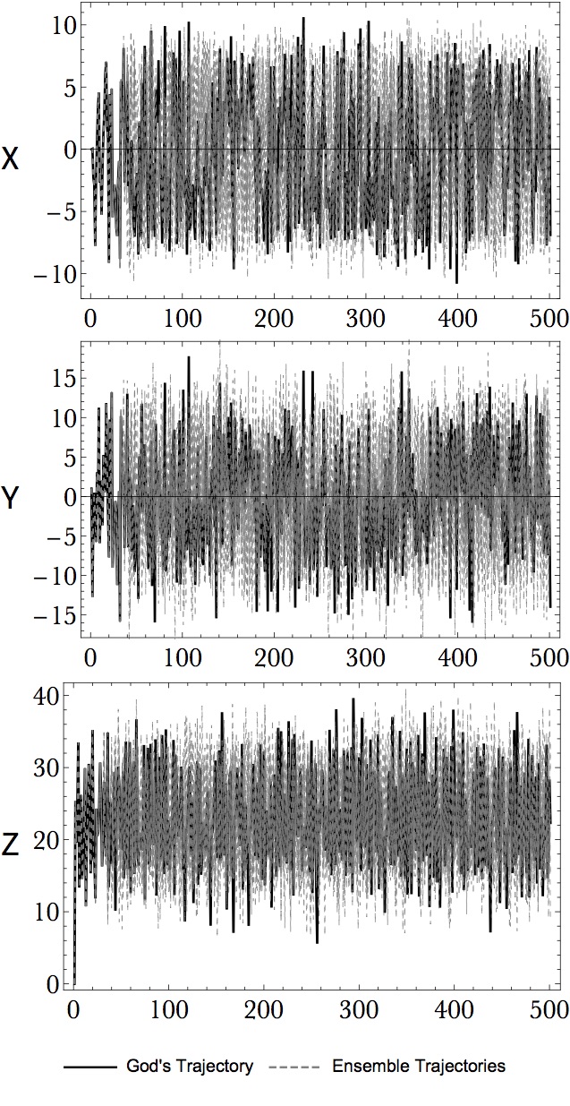
150 samples were generated and evolved for 500 steps, along with the God’s trajectory.

Below I show the projected trajectories on the coordinate planes. Only part of the ensemble members were drawn for clarity.

A very natural question arises that Could Ensemble Forecasts Provide Better Prediction in Deterministic Sense? A general answer to this question is Yes, using ensemble mean:

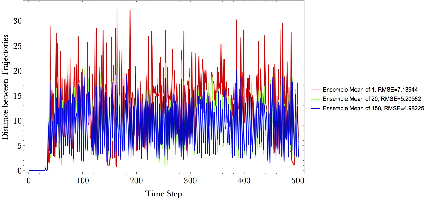
The decease of RMSE is puerly due to statistics rather than any physical improvements. A more detailed exploration will link it to the Law of Large Numbers. We are still faced with the trajectory divergence problem, although the divergence is a liitle bit more converged through averaging ensemble members.

Comparing Lorenz System and Climate System

The Lorenz System above is a pretty simple dynamic system. The Climate System is much more complicated that involves the dynamics and interaction of atmosphere, ocean and landsurface. Also, the climate system is an open system and recieves the forcing from out space and inner geological transitions. However, for certain spatial temporal scale, they are comparable. Relevations can be ignited through the comparison.

With the necessary arguments established above, I can now start

However, Misleading is Worse Than Nothing

Conclusion

Consider that I have the exact initial condition, which is fed to the exact model, and calculated with exact simulation algorithm, I can know both the past and future of a mechanical world. These capacities are named by Roman(Roman, etc.. 2014) as:

1. Observational Omniscience: one is able to determine the true initial condition of the target system.
2. Dynamical Omniscience: one is able to formulate the true time evolution ft of the target system.
3. Computational Omniscience: one is able to calculate the system accurately for any arbitrarily fast.

That information should help water managers to predict what atmospheric rivers may bring. Reservoir engineers in northern California typically release precious water from their reservoirs in the winter, so as to have enough space behind the dam to cope with the threat of flooding. With better knowledge of when atmospheric rivers might arrive and how much water they might carry, says Ralph, engineers should be able to manage that winter release more effectively

It is not complicated, it’s just a lot of it. <div style="text-align: right"> – Richard P. Feynman </div>

###On the Value of Temporal Mean

On the Value of Ensemble